Numerical Integration#
Integration#
The integral of a function \(f(x)\) is evaluated using the fundamental theorem of calculus:
Here, \(F(x)\) is the anti-derivative of \(f(x)\)
Functions for which exact integrals can be computed
Functions for which exact integrals cannot be computed
Numerical Integration#
An intuitive understanding of an integral is:
Numerical integration methods approximate the area under the curve using simple geometrical shapes to evaluate definite integrals
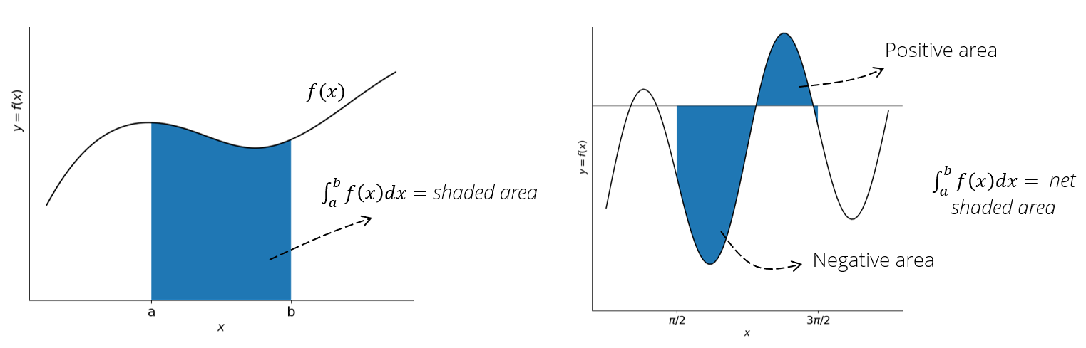
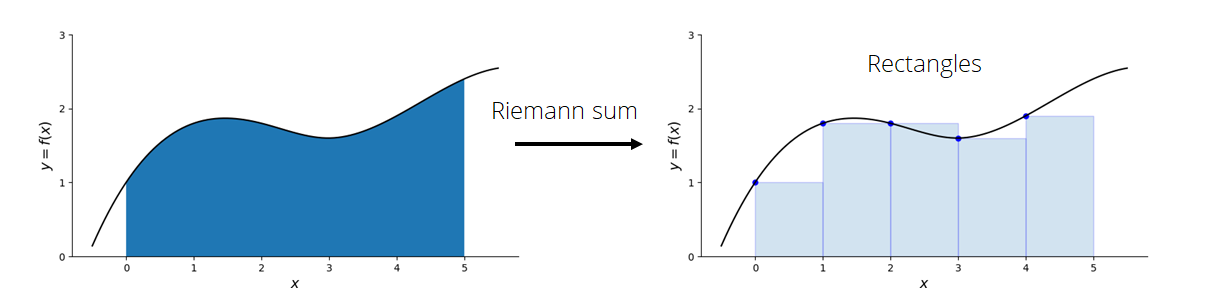
An integral can be approximed by summing the areas of a finite number of subdivisions
Numerical integration methods that use fixed samples of a function:
Reimann sums
Trapezoid rule
Simpson’s rule
These methods do not require the exact function definition
Useful for experimental data
Mathematically, these numercial methods divide the integration domain into sub-domains
The integral is then split into sum of integrals over each sub-domain
Now, the Taylor series approximation of a function around \(x=x_p\)
Substituting this into one of the integral (\(x_i \le x_p \le x_{i+1}\)):
Integrating, we get (\(h = x_{i+1} - x_i\)):
Riemann Sums#
Riemann sums approximate the integrals using just the 1st term of the Taylor series
In other words, Riemann sums assume the function is constant within a subdivision
The subdivision is rectangular in shape
Sum over the curve from \(a\) to \(b\) to approximate the definite integral
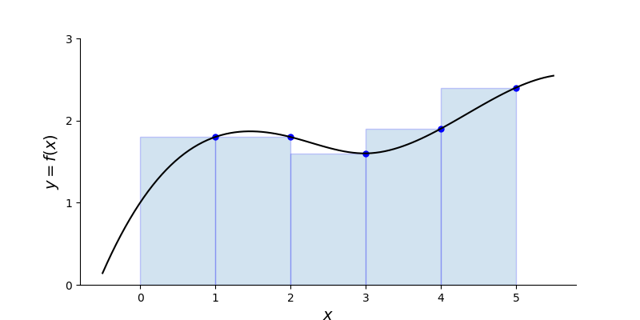
For left Riemann sum:
Uses the left-most point of sub-domain \(x_i\) to compute the height of the rectangle
Right Riemann sum - uses the right-most point \(x_{i+1}\) to compute the height of the rectangle
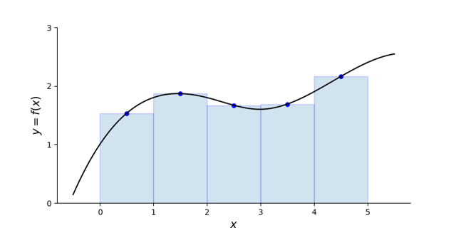
Midpoint Riemann sum - use the mid-point or equivalently, the average of the left and right points
Trapezoid Rule#
The trapezoid rule assumes that the function is linear within the sub-domain
The shape of the area under this linear approximation forms a trapezoid, hence the name
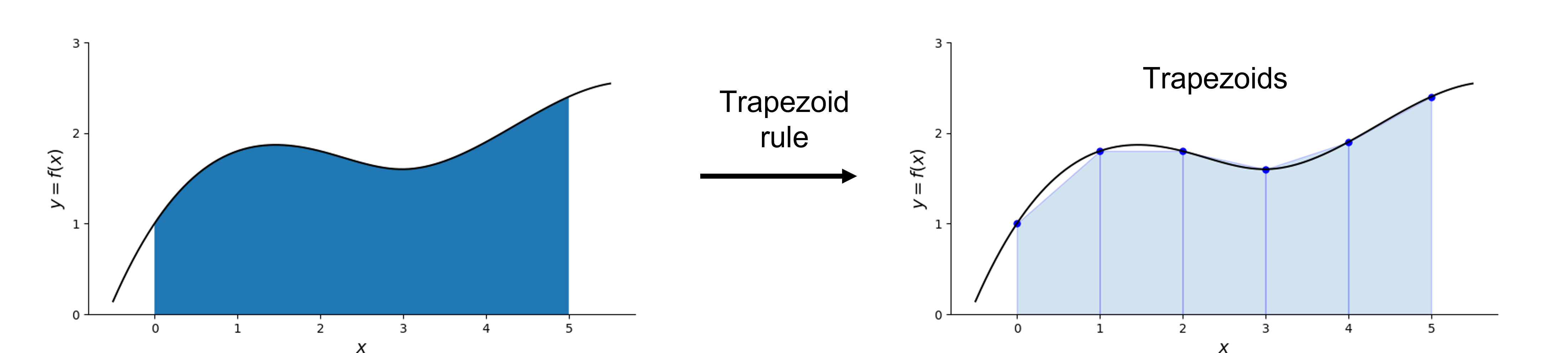
The area for each subdivision is:
Trapezoidal integration is effectively the average of left and right Riemann sums
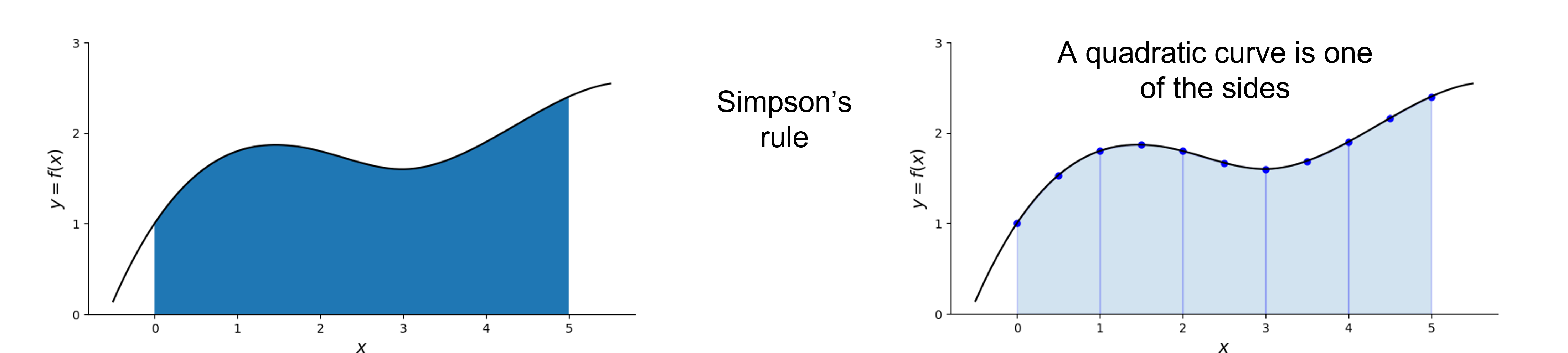
Simpson’s Rule#
Simpson’s rule uses a quadratic function to approximatge the function within a sub-domain consisting of 3 points
Source: https://en.wikipedia.org/wiki/Simpson%27s_rule
According to Simpson’s rule:
Practical Considerations#
The error associated with:
left and right Reimann sums is \(O(h)\)
midpoint Reimann sums and trapezoidal rule is \(O(h^2)\)
Simpson’s rule is \(O(h^4)\)
Often, numerical integration is occuring on sampled experimental data
Thus, the step size is often controlled by the experimental conditions
Use of trapezoidal integration or Simpson’s rule is encouraged to reduce numerical errors
While the error associated with Simpson’s rule is small, it sometimes gives poor results with highly oscillatory functions
Interactive Demonstration#
%matplotlib widget

import numpy as np
from scipy import integrate, interpolate
import matplotlib.pyplot as plt

from ipywidgets import HBox, VBox, interactive, RadioButtons
from IPython.display import display
---------------------------------------------------------------------------
ModuleNotFoundError                       Traceback (most recent call last)
Cell In[1], line 1
----> 1 get_ipython().run_line_magic('matplotlib', 'widget')
      3 import numpy as np
      4 from scipy import integrate, interpolate

File /opt/hostedtoolcache/Python/3.11.9/x64/lib/python3.11/site-packages/IPython/core/interactiveshell.py:2480, in InteractiveShell.run_line_magic(self, magic_name, line, _stack_depth)
   2478     kwargs['local_ns'] = self.get_local_scope(stack_depth)
   2479 with self.builtin_trap:
-> 2480     result = fn(*args, **kwargs)
   2482 # The code below prevents the output from being displayed
   2483 # when using magics with decorator @output_can_be_silenced
   2484 # when the last Python token in the expression is a ';'.
   2485 if getattr(fn, magic.MAGIC_OUTPUT_CAN_BE_SILENCED, False):

File /opt/hostedtoolcache/Python/3.11.9/x64/lib/python3.11/site-packages/IPython/core/magics/pylab.py:103, in PylabMagics.matplotlib(self, line)
     98     print(
     99         "Available matplotlib backends: %s"
    100         % _list_matplotlib_backends_and_gui_loops()
    101     )
    102 else:
--> 103     gui, backend = self.shell.enable_matplotlib(args.gui.lower() if isinstance(args.gui, str) else args.gui)
    104     self._show_matplotlib_backend(args.gui, backend)

File /opt/hostedtoolcache/Python/3.11.9/x64/lib/python3.11/site-packages/IPython/core/interactiveshell.py:3665, in InteractiveShell.enable_matplotlib(self, gui)
   3662     import matplotlib_inline.backend_inline
   3664 from IPython.core import pylabtools as pt
-> 3665 gui, backend = pt.find_gui_and_backend(gui, self.pylab_gui_select)
   3667 if gui != None:
   3668     # If we have our first gui selection, store it
   3669     if self.pylab_gui_select is None:

File /opt/hostedtoolcache/Python/3.11.9/x64/lib/python3.11/site-packages/IPython/core/pylabtools.py:338, in find_gui_and_backend(gui, gui_select)
    321 def find_gui_and_backend(gui=None, gui_select=None):
    322     """Given a gui string return the gui and mpl backend.
    323
    324     Parameters
   (...)
    335     'WXAgg','Qt4Agg','module://matplotlib_inline.backend_inline','agg').
    336     """
--> 338     import matplotlib
    340     if _matplotlib_manages_backends():
    341         backend_registry = matplotlib.backends.registry.backend_registry

ModuleNotFoundError: No module named 'matplotlib'
def numerical_int(f, a, b, N, method='Riemann'):
    '''Compute the Riemann sum of f(x) over the interval [a,b].

    Parameters
    ----------
    f : function -- Vectorized function of one variable
    a , b : float -- Endpoints of the interval [a,b]
    N : int -- Number of subintervals of equal length in the partition of [a,b]
    method : str -- Integration method; valid values 'Riemann', 'Trapezoid' or 'Simpsons'

    Returns
    -------
    float -- Approximation of the integral
    '''
    h = (b - a)/N
    x = np.linspace(a,b,N+1)

    if method == 'Riemann':
        x_mid = (x[:-1] + x[1:])/2
        return h*np.sum(f(x_mid))
    elif method == 'Trapezoid':
        return 0.5*h*np.sum(f(x[:-1]) + f(x[1:]))
    elif method == 'Simpsons':
        return (h/3)*np.sum(f(x[0:-1:2]) + 4*f(x[1::2]) + f(x[2::2]))
    else:
        raise ValueError("Method must be 'Riemann', 'Trapezoid' or 'Simpsons'.")
# Formatting stuff
fs = 20
ls = 20
lw = 2
ms = 10

# x values - global scope
x = np.linspace(-4, 4, 100)

# Radio button for choosing the function
funcButton = RadioButtons(options=['Quadratic'],
                       value='Quadratic',
                       layout={'width': 'max-content'}, # If the items' names are long
                       description='Integrand', disabled=False)

fig, ax = plt.subplots(figsize=(10, 10))

# Interactive plot function callback
def plot_func(IntMeth, Function, N=2):
    # Clear figure
    ax.clear()

    # Set function
    f = None
    fIntExact = None
    titleText = None
    if Function == 'Quadratic':
        f = lambda x: 5 - 0.25*x**2
        fIntExact = 56/3
        titleText = r"$(5 - 0.25x^2)$"
    elif Function == 'Cubic':
        f = lambda x: 5 - 0.1*x**3
        fIntExact = 20
        titleText = r"$(5 - 0.1x^3)$"
    elif Function == 'Quartic':
        f = lambda x: 5 - 0.025*x**4
        fIntExact = 19.68
        titleText = r"$(5 - 0.025x^4)$"
    elif Function == 'Exponential':
        f = lambda x: np.exp(0.1*x)
        fIntExact = 20*np.sinh(0.2)
        titleText = r"$e^{0.1x}$"
    elif Function == 'Cos':
        f = lambda x: np.cos(1.4*np.pi*x)
        fIntExact = np.sin(2.8*np.pi)/0.7/np.pi
        titleText = r"$cos(1.4 \pi x)$"

    # Integration bounds
    a = -2
    b = 2

    # Numerical integrated value
    fInt = numerical_int(f, a, b, N, IntMeth)
    err = (fInt/fIntExact - 1)*100
    ax.set_title(r"$\int_a^b $" + titleText + r"$ dx \approx $" + f"{fInt:4.4f}\nError = {err:4.2f}%\n", fontsize=fs)

    # Line plot of the function
    ax.plot(x, f(x), 'black', lw=lw)
    ax.set_xlabel('$\it{x}$', fontsize=fs)
    ax.set_ylabel('$f(x)$', fontsize=fs)
    #ax.set_xlim(0,6)
    #ax.set_ylim(-1, 110)
    ax.tick_params(axis='both', labelsize=ls)

    # Geometry used for integration
    xSam = np.linspace(-2, 2, N+1)
    if IntMeth == 'Riemann':
        x_mid = (xSam[:-1] + xSam[1:])/2 # Midpoints
        y_mid = f(x_mid)
        ax.plot(x_mid, y_mid, 'b.', markersize=ms)
        ax.bar(x_mid, y_mid, width=4/N, alpha=0.2, edgecolor='b', color='tab:blue')
    elif IntMeth == 'Trapezoid':
        for i in range(N):
            x0 = xSam[i]
            x1 = xSam[i + 1]
            ax.plot(xSam, f(xSam), 'b.', markersize=ms)
            ax.fill_between([x0, x1],[f(x0), f(x1)], color='tab:blue', alpha=0.2, edgecolor='b')
    else:
        for i in range(N//2):
            x0 = xSam[2*i]
            x1 = xSam[2*i + 2]
            xm = xSam[2*i + 1]
            [y0, ym, y1] = [f(x0), f(xm), f(x1)]
            xp = np.linspace(x0, x1, 20)
            h = xm-x0
            yp = (y0/(2*h**2))*(xp-xm)*(xp-x1) \
               - (ym/(  h**2))*(xp-x0)*(xp-x1) \
               + (y1/(2*h**2))*(xp-xm)*(xp-x0)
            ax.plot(xSam, f(xSam), 'b.', markersize=ms)
            ax.fill_between(xp, yp, color='tab:blue', alpha=0.2, edgecolor='b')

    fig.canvas.draw_idle()
    #fig.canvas.flush_events()
    plt.show()

interactive_plot = interactive(plot_func, N=(2, 16, 2),
                                          IntMeth=['Riemann', 'Trapezoid', 'Simpsons'],
                                          Function=['Quadratic', 'Cubic', 'Quartic', 'Exponential', 'Cos'])
output = interactive_plot.children[-1]
output.layout.height = '1200px'

#buttons.observe(updateF, names='value')
display(interactive_plot)
Gauss Integration#
Provides numerical integration rules specialized for polynomials
Also known as Gausian quadrature
\(w_{in} = \) integration weights
\(\zeta_{in} = \) integration points
\(n = \) number of Gauss integration points \((\geq 1)\)
It can be shown that with \(n\) integration points, choosing the integration points to be the roots of the degree-\(n\) Legendre polynomial, \(P_n(x)\) gives exact results for polynomials of order \(2n-1\) (Gauss-Legendre quadrature)
Integrating with scipy.integrate#
The
integratesub-module of scipy provides various functions for numerical integrationIntegration using samples
trapezoid- same astrapzfrom numpysimpsoncumulative_trapezoid- returns a numpy array with integral evaluated as a function of x
Integration when a function object is available
fixed_quad- integration using Gaussian quadraturequad- integration using adaptinve quadrature methodsdblquad,tplquad- double and triple integrationnquad- higher order integration with arbitrary number of variables
Example: evaluate \( \int\limits_o^\pi sin(x) dx \)
from scipy import integrate

# 20 samples of sin(x)
x = np.linspace(0, np.pi, 20)
y = np.sin(x)
# Exact solution
int_exact = -np.cos(np.pi) + np.cos(0)
# numerical integration
int_t = integrate.trapezoid(y, x)
int_s = integrate.simpson(y, x)

print(f'{"Exact: ":>16}{int_exact}\n{"Trapezoid Rule: ":>16}{int_t}\n{"Simpson`s Rule: ":>16}{int_s}')
If \(f(x)\) is the input, then
cumulative_trapezoidfunction computes samples of the integrated function
Example:
x = np.linspace(0, np.pi, 20)
y = np.sin(x)

# Cumulative integration with initial value (a) = 0
y_int = integrate.cumulative_trapezoid(y, x, initial=0)
# For plotting exact value
x_e = np.linspace(0, np.pi, 200)
y_e = np.sin(x_e)
y_int_e = 1 - np.cos(x_e)

# Plot
fig, ax = plt.subplots()
ax.plot(x_e, y_e, '-k', label='sin(x)')
ax.plot(x_e, y_int_e, '-r', label='$\int_0^x sin(x)dx = 1-cos(x)$')
ax.plot(x, y_int,'or', markersize=3, label='Cum. Trapezoid')
ax.set_xlabel('x')
ax.legend();
Scipy Integration#
Integration given function objects
quad,fixed_quad,dblquad,tplquad,nquad
Example: evaluate \(\int\limits_0^{\pi} sin(x) dx\)
The exact value is 2
def f(x):
    return np.sin(x)

integrate.fixed_quad(f, 0, np.pi, n=5)
(2.0000001102844727, None)
The first value in the output
tupleis the integralThe second value is alway
None
# Adaptive Gauss-Kronrod quadrature
integrate.quad(f, 0, np.pi)
(2.0, 2.220446049250313e-14)
The first value in the output
tupleis the integralThe second value is the estimated error
Example: evaluate \(\int\limits_0^\infty e^{-x^2} dx\)
Mathemeticians have defined a special function called the error function because this integral appear fairly commonly:
def f(x):
    return np.exp(-x**2)

# Using Gauss quadrature
val = integrate.quad(f, 0, np.inf)
print(val[0])
0.8862269254527579
from scipy.special import erf

# using the error function
val2 = np.sqrt(np.pi)/2*erf(np.inf)
print(val2)
0.8862269254527579