Root Finding and Optimization#
Root Finding#
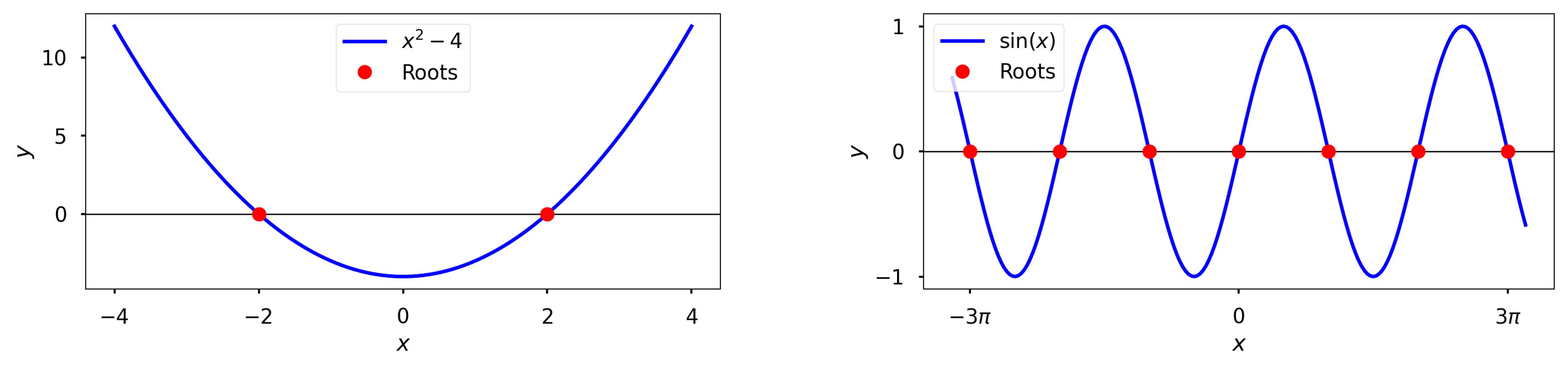
Roots or zeros of a function \(f(x)\) are points where the function assumes a value of zero
Mathematically, roots are all 𝑥 that satisfy \(𝑓(𝑥)=0\)
Examples:
Roots of \(𝑓(𝑥)=𝑥^2−4\) are −2 and 2
\(𝑓(𝑥)=sin(𝑥)\) has infinitely many roots
Roots of simple functions can be found analytically
Quadratic Equation \(ax^2 + bx + c = 0\) $\( x = \frac{-b \pm \sqrt{b^2 - 4ac}}{2a} \)$
Cubic equation \(ax^3 + bx^2 + cx + d = 0\)
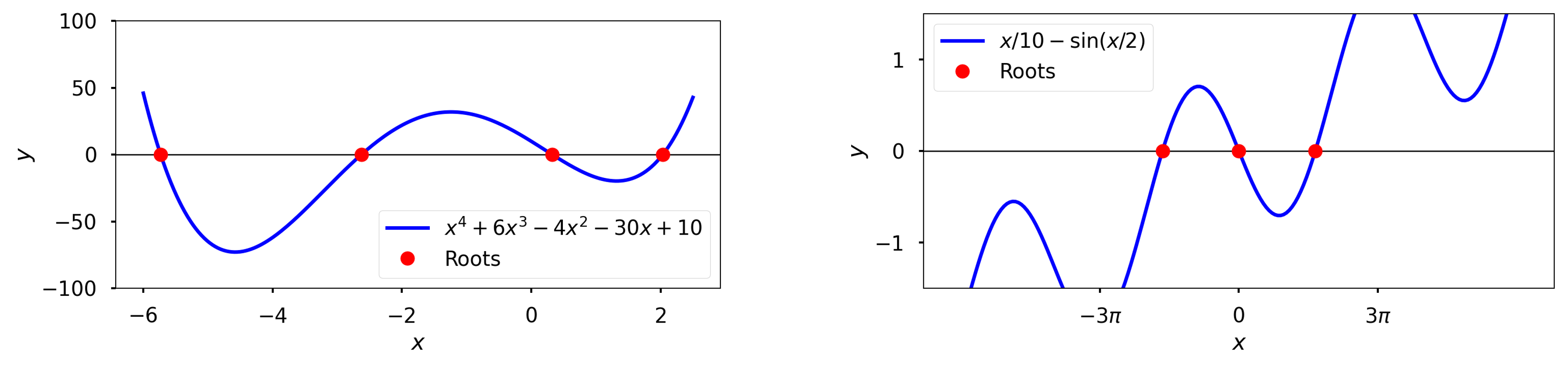
More complicacted functions need a numerical approach
There is no general algorithm for polynomials of order 4 or higher
Implicit equations of some variable can be recast into root finding problems
Example: \(\frac{x}{10} = sin\left(\frac{x}{2} \right)\)
Solution is the same as finding the roots of the function \(f(x) = \frac{x}{10} - sin\left(\frac{x}{2} \right)\)
Algorithms#
Brute Force
Find the value of \(f(x)\) at a large number of points
Can be extremely slow
Bisection method
Iteratively searches for the root by halving the initial search interval/bracket until the interval is small enough and/or \(f(x)\) is small
Easy to implement, but slow
Belongs to a class of methods known as bracketing methods
Only finds one solution even if multiple exist
Newton’s method (a.k.a. Newton-Raphson method)
Uses derivative information to iteratively improve an initial guess for the root
Fast but requires the derivative of the function
Needs an inital guess and does not guarantee that an existing solution will be found
Secant method
Derivative-free version of Newton’s method
Uses finite difference approximation for the derivative
Bisection Method#
Theory#
Intermediate value theorem
If \(f(x)\) is a continuous function in the interval \([a, b]\), then the function takes every values between \(f(a)\) and \(f(b)\)
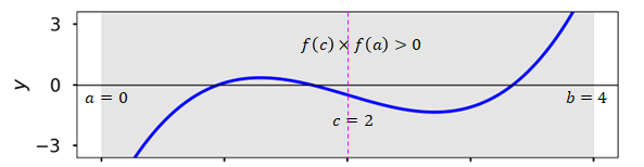
Corollary: if \(f(a) \times f(b) \lt 0\) (i.e., \(f\) has opposite signs at \(x=a\) and \(x=b\)), then there exists at least one root in the interval \([a,b]\)
Bisection method uses this corollary to iteratively search for a root
Algorithm#
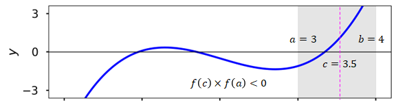
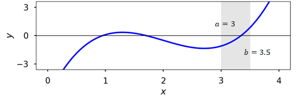
Pick an interval \([a,b]\) such that \(f(a)\times f(b) < 0\)
Compute \(f(c)\) where \(c = \frac{a+b}{2}\) is the interval midpoint
Check if \(f(c) \leq \epsilon\) where \(\epsilon << 1\) is the tolerance
If true, stop the algorithm
Else, continue
This is referred to as the stopping criterion (or criteria)
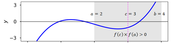
If \(f(c)\times f(a) > 0\), reject the subinterval \([a,c]\) and go to step 2 with \(a\) replaced by \(c\)
Else, reject the subinterval \([c,b]\) and go to step 2 with \(b\) replaced by \(c\)
Visualization#
Implementation#
%matplotlib widget
import numpy as np
import matplotlib.pyplot as plt

def bisection(f, a, b, tol=1e-4):
    fa = f(a)
    fb = f(b)
    if fa*fb > 0:
        raise Exception("f(a)*f(b) > 0")

    #midpoint
    c = 0.5*(a+b)
    fc = f(c)

    #iterations
    it = 1
    itData = [[a,b]]
    while abs(fc) > tol:
        if fa*fc > 0:
            a = c
            fa = fc
        else:
            b = c
        c = 0.5*(a+b)
        fc = f(c)
        it += 1
        itData += [[a,b]]

    return c, np.array(itData)
---------------------------------------------------------------------------
ModuleNotFoundError                       Traceback (most recent call last)
Cell In[1], line 1
----> 1 get_ipython().run_line_magic('matplotlib', 'widget')
      2 import numpy as np
      3 import matplotlib.pyplot as plt

File /opt/hostedtoolcache/Python/3.11.9/x64/lib/python3.11/site-packages/IPython/core/interactiveshell.py:2480, in InteractiveShell.run_line_magic(self, magic_name, line, _stack_depth)
   2478     kwargs['local_ns'] = self.get_local_scope(stack_depth)
   2479 with self.builtin_trap:
-> 2480     result = fn(*args, **kwargs)
   2482 # The code below prevents the output from being displayed
   2483 # when using magics with decorator @output_can_be_silenced
   2484 # when the last Python token in the expression is a ';'.
   2485 if getattr(fn, magic.MAGIC_OUTPUT_CAN_BE_SILENCED, False):

File /opt/hostedtoolcache/Python/3.11.9/x64/lib/python3.11/site-packages/IPython/core/magics/pylab.py:103, in PylabMagics.matplotlib(self, line)
     98     print(
     99         "Available matplotlib backends: %s"
    100         % _list_matplotlib_backends_and_gui_loops()
    101     )
    102 else:
--> 103     gui, backend = self.shell.enable_matplotlib(args.gui.lower() if isinstance(args.gui, str) else args.gui)
    104     self._show_matplotlib_backend(args.gui, backend)

File /opt/hostedtoolcache/Python/3.11.9/x64/lib/python3.11/site-packages/IPython/core/interactiveshell.py:3665, in InteractiveShell.enable_matplotlib(self, gui)
   3662     import matplotlib_inline.backend_inline
   3664 from IPython.core import pylabtools as pt
-> 3665 gui, backend = pt.find_gui_and_backend(gui, self.pylab_gui_select)
   3667 if gui != None:
   3668     # If we have our first gui selection, store it
   3669     if self.pylab_gui_select is None:

File /opt/hostedtoolcache/Python/3.11.9/x64/lib/python3.11/site-packages/IPython/core/pylabtools.py:338, in find_gui_and_backend(gui, gui_select)
    321 def find_gui_and_backend(gui=None, gui_select=None):
    322     """Given a gui string return the gui and mpl backend.
    323
    324     Parameters
   (...)
    335     'WXAgg','Qt4Agg','module://matplotlib_inline.backend_inline','agg').
    336     """
--> 338     import matplotlib
    340     if _matplotlib_manages_backends():
    341         backend_registry = matplotlib.backends.registry.backend_registry

ModuleNotFoundError: No module named 'matplotlib'
def func(x):
    return 1.2*x**3 - 7.2*x**2 + 12.6*x - 6.5

root, itData = bisection(func, 1, 2.5, tol=0.01)
print(root, itData, sep='\n')
x = np.linspace(0, 4, 200)
y = func(x)

xRoot = (itData[-1][0] + itData[-1][1])*0.5
yRoot = func(xRoot)

fig, ax = plt.subplots(1, 1, figsize=(6, 2.5))
ax.plot(x, y, '-b')
ax.plot([xRoot], [yRoot], 'or')
ax.axhline(y=0, color='k', lw=1)
ax.set_xlabel('$x$')
ax.set_ylabel('$y$')
ax.set_xticks(np.linspace(0, 4, 5))
ax.set_yticks(np.linspace(-3, 3, 3))
ax.set_ylim(-3.6, 3.6)
plt.tight_layout();
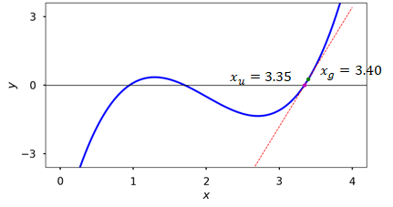
Newton’s Method#
Theory#
Let \(f(x)\) be a smooth continuous function
Using the Taylor series, the linear approximation of the function at a point \(x = x_0\) is:
For root finding:
Repeatedly applying this formula leads to a root of \(f(x)\) if the iterations do not diverge due to \(f'(x_i) = 0\)
Algorithm#
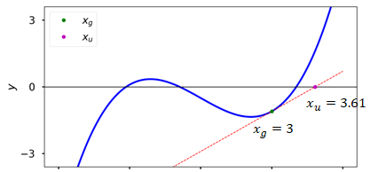
Pick an initial guess \(x_g\) for the root of \(f(x)\)
Check if \(f(x_g)\epsilon\) where \(\epsilon\) is the tolerance
If true, stop the iterations
Compute \(f'(x_g)\)
If \(f'(x_g) = 0\), terminate with an error
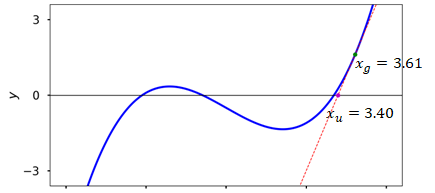
Update the guess using:
Replace \(x_g\) with \(x_u\) and go to step 2
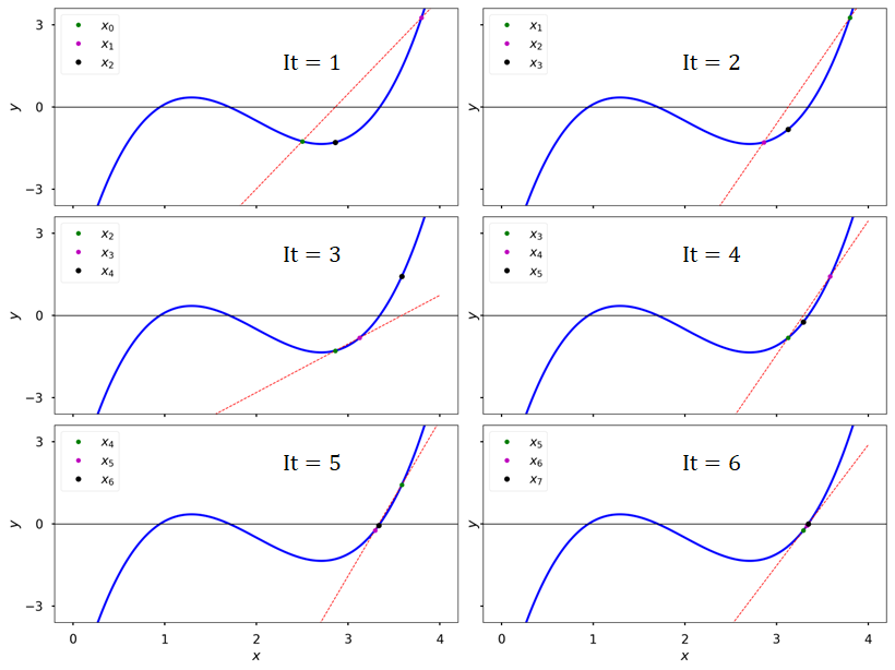
Visualization#
Implementation#
def newton_method(f, df, xg, eps=1.e-4, itMax=10):
    hist = [xg]
    it = 0
    x=xg
    while it <= itMax:
        dfdx = df(x)
        if abs(dfdx) < 1.e-6:
            raise Exception("Zero derivative encountered")
        x = x - f(x)/df(x)
        it += 1
        hist += [x]
        if abs(f(x)) < eps:
            break

    return hist

def f(x):
    return 1.2*x**3 - 7.2*x**2 + 12.6*x - 6.5

def dfdx(x):
    return 3.6*x**2 - 14.4*x + 12.6

hist_newton = newton_method(f,dfdx,3)
print(hist_newton)
Secant Method#
Theory#
Uses secant lines instead of tangent lines
Secant lines are lines that cut a curve at a minimum of 2 distinct points
In the Newton’s method formula, we replace \(f'(x)\) with its finite difference (FD) approximation
The algorithm uses the last two guesses to compute the FD approximation and the updated guess:
\[ x_{n+1} = x_n - f(x_n)\frac{x_n - x_{n-1}}{f(x_n) - f(x_{n-1})} \]
Visualization#
Implementation#
def secant_method(x0, x1, tol=1e-4, max_iter=100):
    hist = [x0,x1]
    for i in range(max_iter):
        fx0, fx1 = f(x0), f(x1)
        x2 = x1 - fx1 * (x1 - x0) / (fx1 - fx0)
        hist.append(x2)
        if abs(x2 - x1) < tol:
            return hist
        x0, x1 = x1, x2
    raise ValueError("The method failed to converge.")


def f(x):
    return 1.2*x**3 - 7.2*x**2 + 12.6*x - 6.5

# Initial guesses
x0, x1 = 3, 4

# Find the root of the function
root = secant_method(x0, x1)
print(root)
Root finding in Scipy#
root_scalar
Function in scipy’s
optimizesubmodule for finding roots of 1D functionsAutomatically chooses an appropriate algorithm based on inputs
Algorithm can be explicitly chosen through the
methodkeyword argumentbrentqis the best to use if a bracket is providedIf derivative is provided,
newtonis better
from scipy import optimize

def f(x):
    return 1.2*x**3 - 7.2*x**2 + 12.6*x - 6.5

optimize.root_scalar(f, bracket = (2,4), method = 'brentq')
def dfdx(x):
    return 3.6*x**2 - 14.4*x + 12.6

optimize.root_scalar(f, x0=3, fprime = dfdx, method = 'newton')
Optimization#
Optimization is concerned with determining the best outcome of a prescribed objective given a set of constraints
Also called mathematical programming in the operations research community where many optimization methods have been developed
Here, programming refers to planning and scheduling
Engineering often requires design optimization
Design goals are quantified using model functions and constraints
Typically, this process involves trade-offs between multiple optimization goals
Classification of optimization problems
Based on existence of constraints
Unconstrained
Constrained
Based on nature of functions
Linear programming problem
Objective and constraint functions are linear in design variables
Quadratic programming problem
Objective is quadratic
Constraints are linear
Nonlinear programming (NLP) problem
One of objective or constraints is a non-linear function
Most general case; linear and quadratic programming are special cases
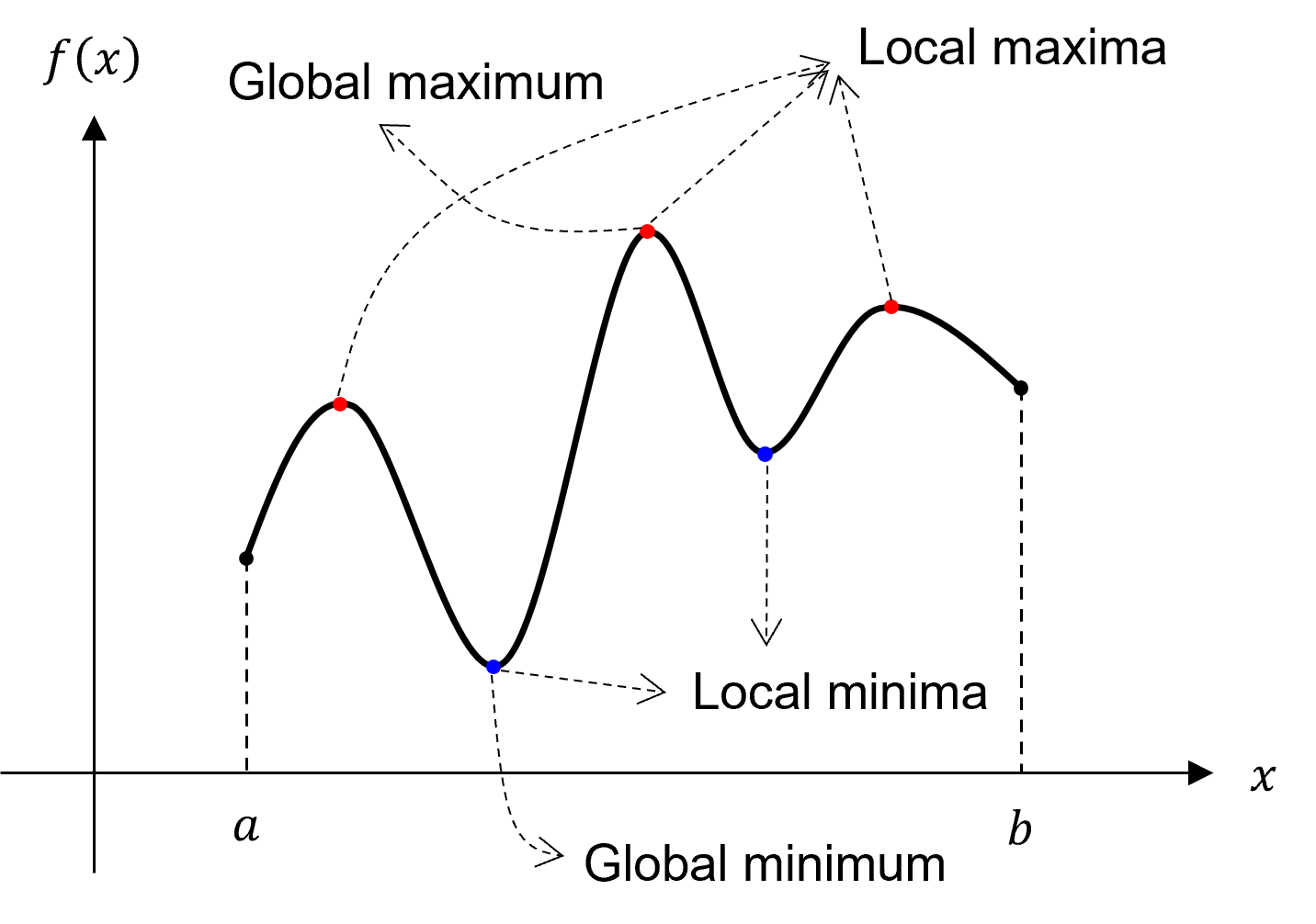
Unconstrained Optimization#
Optimization is concerned with finding local/global maxima and minima of a function
Maximizing some function \(f\) is equivalent to minimizing the function \(-f\)
Maxima and minima are found where the derivative at some point, \(x_i\), is \(f'(x_i) = 0\)
Necessary condition
The second derivative is required to determine if the point is a maximum, a minimum, or neigher
Local minima if \(f''(x_i) > 0\)
Local maxima if \(f''(x_i) < 0\)
Sufficient condition
Numerical approaches:
Local methods:
Find a solution that satisfy the necessary and sufficient conditions
Can only find a local minimum (or maximum)
Global methods:
Algorithms that attempt to find a global minimum (or maximum)
1D local methods
Elimination methods (0th order methods)
Bracketing method
Fibonacci method
Golden section method
\(\cdots\)
Interpolation methods
Quadratic method (0th order)
Davidon’s cubic method (1st order)
Newton’s method (2nd order)
\(\cdots\)
\(n\)D local methods
Direct methods (0th order methods)
Univariate search
Hooke-Jeeves method
Nelder-Mead or sequential simplex method
Powell’s conjugate directions method
\(\cdots\)
Indirect methods (1st and 2nd order methods)
Steepest descent
Conjugate gradient (CG) method
Newton’s method
Quasi-Newton methods
Davidon-Fletcher-Powell (DFP) method
Broyden-Fletcher-Goldfarb-Shanno (BFGS) method
\(\cdots\)
Optimization in Scipy#
Optimization functions
minimize_scalarFind the minimum of a 1D function in a given interval
Only support bracketing and golden section methods
minimizeMultidimensional variant
Supports:
Nelder-Mead
Powell
Conjugate gradient (CG)
BFGS
COBYLA
SLSQP
Himmelblau’s function is designed to test the performance of optimization algorithms
# define the himmelblau function
def himmelblau(x):
    return (x[0]**2 + x[1] - 11)**2 + (x[0] + x[1]**2 - 7)**2

# optimize
optimize.minimize(himmelblau, x0 = np.array([0, 0]), method = 'Powell')
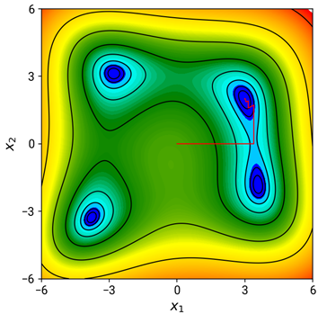
# set the initial guesses for the local minima
x0_list = [
    np.array([-4, -4]),
    np.array([4, -4]),
    np.array([-4, 4]),
    np.array([4, 4])
]

# use minimize with the Nelder-Mead method to find each local minimum
for i, x0 in enumerate(x0_list):
    res = optimize.minimize(himmelblau, x0, method='Nelder-Mead')
    x = res.x
    f_val = res.fun
    print(f"Local minimum {i+1} at x = {x}, f(x) = {f_val}")