Linear Algebra#
Scipy Modules#
Scipy has two main linear algebra modules:
scipy.linalgandscipy.sparse.linalgscipy.sparse.linalghas specialized algorithms for sparse matrices
Dense matrix example
Majority matrix elements are non-zero
Sparse matrix example
Only 11 out of 64 matrix elements are non-zero
Both
scipy.linalgandscipy.sparse.linalgare interfaces to two standard librariesBLAS - basic linear algebra subprograms
Contains optimized routines for vector addition, dot products, matrix multiplication etc.
LAPACK - linear algebra package
Implements optimized routines for matrix decompositions/factorizations, solving linear systems, eigenvalue problems, and linear least squares
Functions provided by
scipy.linalgBasic functions –
det,inv,pinv, …Linear system solvers -
solve,solve_banded,solve_triangular,lstsq, \(\cdots\)Eigenproblem solvers –
eig,eigvals,eig_banded,eigvals_banded, \(\cdots\)Matrix decompositions –
lu,qr,cholesky,schur, \(\cdots\)
Pseudoinverse of a Matrix#
For a non-singular square matrix \(A\), the inverse \(A^{-1}\) satisfies:
Moore-Penrose pseudo-inverse \(A^+\) of a matrix \(A\) satisfies:
\(A^+\) exists for any matrix - including singular and non-square matrices
For matrices with linearly independent rows (right inverse):
For matrices with linearly independent columns (left inverse):
For non-singular square matrices, this simplifies to \(A^+ = A^{-1}\) in both cases
The pseudo-inverse’s dimensions are \(n \times m\) if the matrix \(A\) has dimensions \(m \times n\)
pinvfromscipyslinalgmodule can be used to compute the pseudo-inverse
import numpy as np
from scipy import linalg

A = np.array([[ 1, 4, 3, 2],
              [ 3, 5, 2, 1],
              [-1, 0, 6, 0]])

print(repr(linalg.pinv(A))) # Right inverse
---------------------------------------------------------------------------
ModuleNotFoundError                       Traceback (most recent call last)
Cell In[1], line 1
----> 1 import numpy as np
      2 from scipy import linalg
      4 A = np.array([[ 1, 4, 3, 2],
      5               [ 3, 5, 2, 1],
      6               [-1, 0, 6, 0]])

ModuleNotFoundError: No module named 'numpy'
B = np.array([[1, 3], [2, 6], [4, 7]])
print(repr(linalg.pinv(B))) # Left inverse
array([[-0.28, -0.56,  0.6 ],
       [ 0.16,  0.32, -0.2 ]])
Linear System of Equations#
A linear system of equations are a set of \(m\) linear equations in \(n\) variables \(x_1, x_2, \cdots, x_n\)
In matrix form:
To determine \(x\), we can use the inverse if \(m=n\) and all rows are linearly independent:
This is computationally inefficent
More efficient algorithms
Gauss elimination
Gauss-Jordan elimination
LU decomposition
Cholesky decomposition
Scipy uses LU decomposition by default
Cholesky decomposition is used if the matrix \(A\) is symmetric and positive-definite
If the number of equations is not the same as the number of unknowns, i.e., \(m \ne n\), we can use the
lstsqfunctionThe least squares algorithm computes the vector \(x\) that minimizes the least squares error \(\lvert b - Ax \rvert\)
It can be shown that the \(x\) that minimizes \(\lvert b - Ax \rvert\) is given by:
Here \(A^+\) is the pseudo-inverse of \(A\)
A = np.array([[ 1, 4, 3, 2],
              [ 3, 5, 2, 1],
              [-1, 0, 6, 0]])
b = np.array([2, 1, -2])
res = linalg.lstsq(A, b)
res
(array([-0.4593519 ,  0.45110858, -0.40989198,  0.94229676]),
 array([], dtype=float64),
 3,
 array([8.63395251, 5.46582073, 1.25684835]))
x = res[0]
(A @ x - b).round(4)
array([-0., -0., 0.])
A = np.array([[1, 3],
              [2, 6],
              [4, 7]])
b = np.array([1, 2, 3])
res = linalg.lstsq(A, b)
res
(array([0.4, 0.2]),
 6.943647297459356e-32,
 2,
 array([10.67251474,  1.04758252]))
x = res[0]
(A @ x - b).round(4)
array([-0., -0., -0.])
Consider some data collected from experiments
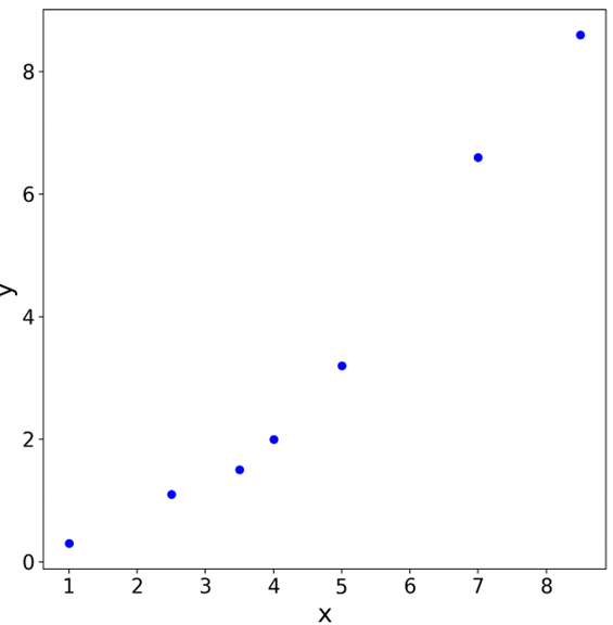
We want to fit this data to a quadratic curve (hypothesis) of the form \(a_1 + a_2 x + a_3 x^2\)
We can obtain the unknown coefficients \(a_1\), \(a_2\) and \(a_3\) by solving the linear system formed by the observed data
x = np.array([1, 2.5, 3.5, 4, 5, 7, 8.5])
y = np.array([0.3, 1.1, 1.5, 2.0, 3.2, 6.6, 8.6])
M = x.reshape(x.size, 1)**[0, 1, 2]
M
array([[ 1.  ,  1.  ,  1.  ],
       [ 1.  ,  2.5 ,  6.25],
       [ 1.  ,  3.5 , 12.25],
       [ 1.  ,  4.  , 16.  ],
       [ 1.  ,  5.  , 25.  ],
       [ 1.  ,  7.  , 49.  ],
       [ 1.  ,  8.5 , 72.25]])
res = linalg.lstsq(M, y)
res
(array([0.0578403 , 0.07701453, 0.11262261]),
 0.3954624919193902,
 3,
 array([94.14628205,  4.12516865,  0.63091939]))
linalg.pinv(M) @ y
array([0.0578403 , 0.07701453, 0.11262261])
%matplotlib widget
import matplotlib.pyplot as plt

fig, ax = plt.subplots()
ax.plot(x, y, 'ob', label='data')
a = res[0]
xx = np.linspace(0, 9, 101)
yy = a[0] + a[1]*xx + a[2]*xx**2
ax.plot(xx, yy, '-r', label='least squares fit, $y = a_1 + a_2x + a_3x^2$')
ax.set_xlabel('x', fontsize=20)
ax.set_ylabel('y', fontsize=20)
ax.legend(fontsize=14)
ax.tick_params(labelsize=16)
fig.set_size_inches(8, 8)
Solving Linear Systems#
Numerical approaches to solving linear system of equations
Direct solvers
Use methods based on eliminations that lead to matrix decomposition or factorization
Matrix decompositions
LU decomposition
Cholesky decomposition
Eigen decomposition
QR decomposition
\(\cdots\)
Indirect solvers
Start with a guess and iteratively improve the guess
Methods
Jacobi
Gauss-Seidel
Sparse indirect solvers - Conjugate Gradient (CG), BIConjugate Gradient (BiCG), Generalized Minimum RESidual (GMRES), …
Direct Solvers#
The solution of linear system \(Ax=b\) is straightforward if the coefficient matrix \(A\) has a special form (diagonal, lower or upper triangular forms)
Forward substitution algorithm
Applicable for a lower triangular linear systems \(Lx = b\) where \(L\) is a lower triangular matrix
If any of the diagonal terms are zero, the system is singular \(\rightarrow\) use the least squares method
Backward substitution algorithm
Applicable for an upper triangular linear systems \(Ux = b\) where \(U\) is an upper triangular matrix
The algorithm works bottom up, solving for \(x_n\) first and \(x_1\) in the final step
If any of the diagonal terms are zero, the system is singular \(\rightarrow\) use the least squares method
Gaussian elimination or row reduction
Algorithm for converting a given matrix to an equivalent upper triangular form
Uses 3 kinds of row operations sequentially
Swap the position of rows i and j
Scale row i by a non-zero value \(\alpha\)
Add a row j scaled by a value of \(\alpha\) to row i
Gauss-Jordan elimination
Extends the Gaussian elimination algorithm to convert a matrix to an equivalent diagonal form
Uses the same row operations
Can be used to determine the inverse of a matrix
Gaussian Elimination#
Example:
The augmented matrix
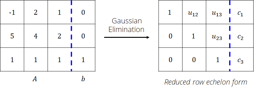
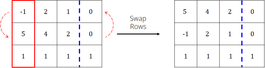
From the 1st column, choose a pivot row
The row with the max absolute value is used
Note: if all the values in the column are zero, then \(A\) is singular and no solution exists
Swap the pivot row with the first row
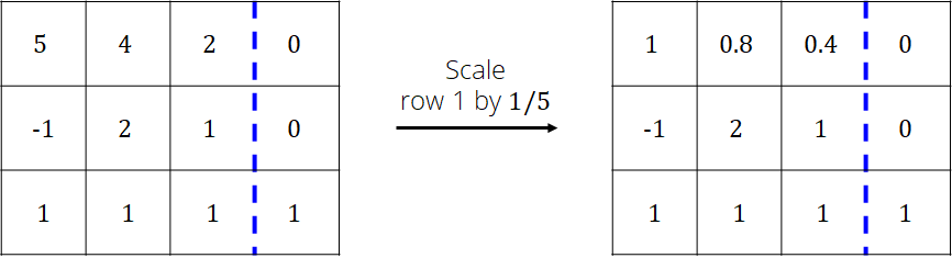
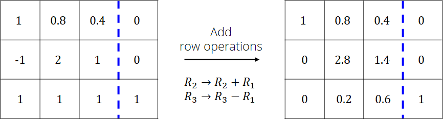
Scale the pivot row (1st row now) so that the value in the 1st column is 1
Add the pivot row to the rows below so that the values in the 1st column are zero
Repeat the procedure with column 2 while ignoring row 1
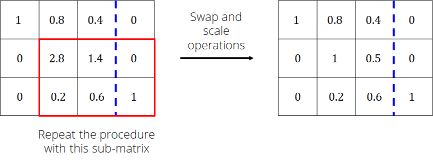
Repeat the procedure with column 2 while ignoring row 1
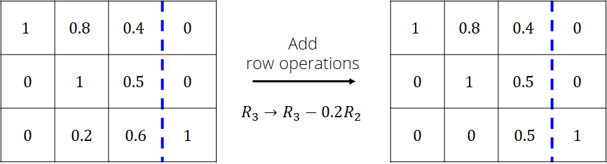
Repeat the procedure with column 3 while ignoring rows 1 and 2
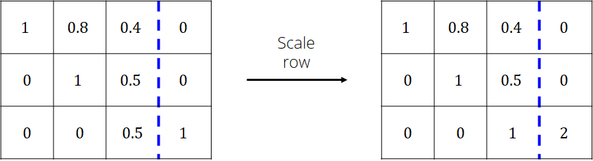
The matrix is now in upper triangle form and can be solved using backward substitution algorithm
%matplotlib widget

import numpy as np
import matplotlib.pyplot as plt
import ipywidgets
from IPython.display import display

def viz_matrices(M1, M2, text=''):
    # Check input
    if not (isinstance(M1, np.ndarray) and isinstance(M2, np.ndarray)):
        raise TypeError("numpy arrays expected")

    # Num rows
    n = M1.shape[0]

    # Width of each cell
    w = 2

    # Create empty figure with three axes
    plt.ioff() # Will not show the figure unless explicitly asked to do so
    #plt.clf() # Clear the current figure
    fig, axs = plt.subplots(1, 3, figsize=(8, 2), gridspec_kw={'width_ratios':[2, 1, 2]})

    # Decorate each axes
    M = [M1, None, M2]
    txtAxes = []
    fs = 6
    for p, ax in enumerate(axs):
        ax.axis('off')

        if p == 1:
            ax.quiver([0], [0], [1], [0], scale_units='x', scale=1, headwidth=12, headlength=10)
            txt = ax.text(0.5, 0.02, text, ha='center', fontsize=8)
            txtAxes.append(txt)
            ax.set_xlim(0, 1.2)
            continue

        # Add grid lines and data from M as text
        for i in range(n):
            ax.plot([0, w*(n+1)], [w*i, w*i], '-k')
            ax.plot([w*i, w*i], [0, w*n], '-k')
            for j in range(n+1):
                txt = ax.text(w*(j + 0.5), w*(n - i - 0.5), f'{M[p][i, j]:6.2f}', ha='center', fontsize=fs)
                txtAxes.append(txt)

        ax.plot([0, w*(n+1)], [w*n, w*n], '-k')
        ax.plot([w*n, w*n], [0, w*n], '--b')
        ax.plot([w*(n+1), w*(n+1)], [0, w*n], '-k')

    #fig.set_size_inches(12, 3)

    return (fig, txtAxes)

def gauss_elim(A, b):
    if not (isinstance(A, np.ndarray) and isinstance(b, np.ndarray)):
        raise TypeError("numpy array expected")

    n = A.shape[0]
    if n != b.shape[0]:
        raise Exception("Incompatible dimensions")

    # Row operation functions
    def scale_row(M, i, a):
        M[i] *= a

    def add_row(M, i, j, a):
        M[i] += a*M[j]

    def swap_row(M, i, j):
        M[[i, j]] = M[[j, i]]

    # Reshape b to a column vector
    b = b.reshape(n, 1)

    # Augmented matrix
    B = np.hstack((A, b))
    print(B, '\n')

    #ax.table(cellText = B, loc='center')

    # Loop over the rows
    for i in range(n):
        # Determine the pivot location
        j = np.argmax(np.abs(B[:, i][i::])) + i

        # Swap rows
        swap_row(B, i, j)

        # Scale row
        scale_row(B, i, 1/B[i,i])

        # Pivoting
        for p in range(i+1, n):
            add_row(B, p, i, -B[p, i])
        print(B, '\n')

    return B

def gauss_elim_interactive(A, b):
    if not (isinstance(A, np.ndarray) and isinstance(b, np.ndarray)):
        raise TypeError("numpy array expected")

    n = A.shape[0]
    if n != b.shape[0]:
        raise Exception("Incompatible dimensions")

    # Row operation functions
    def scale_row(M, i, a):
        M[i] *= a

    def add_row(M, i, j, a):
        M[i] += a*M[j]

    def swap_row(M, i, j):
        M[[i, j]] = M[[j, i]]

    # Reshape b to a column vector
    b = b.reshape(n, 1)

    # Augmented matrix
    B = np.hstack((A, b))

    # Visualization stuff
    ## Create a figure
    fig, txtAxs = viz_matrices(B, B, "Init")

    ## Create button
    button = ipywidgets.Button(description='Next',
                               disabled=False,
                               button_style='', # 'success', 'info', 'warning', 'danger' or ''
                               tooltip='Next',
                               icon='arrow-right') # (FontAwesome names without the `fa-` prefix)
    output = ipywidgets.Output()

    ## Button callback
    global i, opCount
    i = 0 # Keep track of the iterations
    opCount = 0 # Keep track of the row operations
    def update_viz_matrices(button):
        # Needed in order to modify i, opCount
        # Not required if just accessing them
        global i, opCount

        with output:
            Bprev = np.copy(B)
            text = ''

            # Do nothing if reached the last row
            if i >= n:
                button.description = "Algorithm ended!"
                button.disabled = True
                return

            if opCount%3 == 0:
                # Update the augmented matrix
                # Determine the pivot location
                j = np.argmax(np.abs(B[:, i][i::])) + i

                if i != j:
                    # Swap rows
                    swap_row(B, i, j)

                    text = f'Swap rows {i+1} and {j+1}'
                else:
                    text = f'No swapping'

            if opCount%3 == 1:
                text = f'Scale row {i+1} by {B[i,i]:4.2f}'

                # Scale row
                scale_row(B, i, 1/B[i,i])

            if opCount%3 == 2:
                # Pivoting
                for p in range(i+1, n):
                    add_row(B, p, i, -B[p, i])

                if i+1 < n:
                    text = f'Pivot rows {i+2} to {n}'

                else:
                    text = 'Algorithm ended!'

            for c, ax in enumerate(txtAxs):
                if c < n*(n+1):
                    ax.set_text(f'{Bprev[c//(n+1), c%(n+1)]:4.2f}')
                elif c > n*(n+1):
                    ax.set_text(f'{B[(c-1)//(n+1) - n, (c-1)%(n+1)]:4.2f}')
                    if B[(c-1)//(n+1) - n, (c-1)%(n+1)] != Bprev[(c-1)//(n+1) - n, (c-1)%(n+1)]:
                        ax.set_c('r')
                    else:
                        ax.set_c('k')
                else:
                    ax.set_text(text)
            fig.canvas.draw()
            fig.canvas.flush_events()
            opCount += 1
        i = opCount//3

    ## Add callback to the button
    button.on_click(update_viz_matrices)

    ## Box with the figure
    display(ipywidgets.VBox([button, output, fig.canvas]))
A = np.array([[1, 2, 3, 7, 10],
              [13, 4, 5, 12, 15],
              [7, 8, 3, 0, 18],
              [12, 8, 9, 1, 5],
              [10, 1, 9, 8, 7]], dtype=float)

b = np.array([2, 2, 2, 2, 2], dtype=float)

gauss_elim_interactive(A, b)
Matrix Decomposition#
Gaussian elimination is restricted to a specific RHS vector \(b\)
This is disadvantageous when it is required to solve a linear system with the same \(A\) but different RHS vectors
A more efficient approach is decomposition or factorization of a matrix that can be reused for different \(b\)
Matrices once decomposed will simplify the solution procedure for the linear system
Scipy’s matrix decomposition functions:
lu,ldl,svd,cholesky,polar,qr,qz,schur,eig, \(\cdots\)
LU Decomposition#
LU decomposition is based on the matrix form of the Gaussian elimination algorithm
Decomposes the matrix into a product of a lower triangular and an upper triangular matrices, thus the name LU
Some matrices do not possess an LU decomposition
However, a decomposition exists if the rows are permuted
The decomposition in this case looks like \(A = PLU\) where \(P\) is the permutation matrix
Solving a linear system given the LU decomposition
Denoting \(Ux=y\), \(Ax=Ly=b \rightarrow\) solve using forward substitution algorithm
Once \(y\) is known, solve \(Ux=y\) using the backward substitution algorithm for \(x\)
from scipy import linalg

A = np.array([[9, 3, 4],
              [4, 3, 4],
              [1, 1, 1]], dtype=float)

linalg.lu(A)
(array([[1., 0., 0.],
        [0., 1., 0.],
        [0., 0., 1.]]),
 array([[1.        , 0.        , 0.        ],
        [0.44444444, 1.        , 0.        ],
        [0.11111111, 0.4       , 1.        ]]),
 array([[ 9.        ,  3.        ,  4.        ],
        [ 0.        ,  1.66666667,  2.22222222],
        [ 0.        ,  0.        , -0.33333333]]))
Output is a
tupleofndarrays, i.e.,(P, L, U)
Cholesky Decomposition#
Cholesky decomposition is a special case of LU decomposition
Applicable to symmetric positive-definite matrices
Eigen Decomposition#
Eigenvectors \(v\) of a matrix \(A\) are vectors that satisfy (\(\lambda\) are eigenvalues):
If the eigenvectors are linearly independent, then \(A\) can be factorized as:
\(Q\) is a matrix formed by joining the eigenvectors (each column of \(Q\) is an eigenvector)
\(D\) is a diagonal matrix formed by the corresponding eigenvalues
For a symmetric positive-definite matrix, \(Q^{−1} = Q^T\), i.e., \(Q\) is an orthogonal matrix
A = np.array([[9, 3, 4],
              [4, 3, 4],
              [1, 1, 1]], dtype=float)

la, v = linalg.eig(A)
print("Eigenvalues:  ", la.real)
for i in range(3):
    print(f"Eigenvector {i}:", v[:, i])
Eigenvalues:   [11.275622    1.95159452 -0.22721652]
Eigenvector 0: [0.86622734 0.48211224 0.13121732]
Eigenvector 1: [ 0.51375558 -0.80249012 -0.30342182]
Eigenvector 2: [-0.03309737 -0.76141963  0.64741387]
Gauss-Seidel & Jacobi Methods#
Iterative procedures that split the coefficient matrix \(A\) into three parts
The lower triangular part \(L\), the diagonal part \(D\) and the upper triangular part \(U\)
Gauss-Seidel Method#
The linear system is rewritten as:
Assuming the values of \(x=x^{(0)}\) on the RHS and using the forward substitution algorithm, an iterative update scheme is used
Here \(x^{(k)}\) is the vector containing the solution at \(k^th\) iteration
Jacobi Method#
The linear system is rewritten as:
Starting with an initial guess of \(x=x^{(0)}\), the iterative update scheme is:
Gauss-Seidel method converges if \(A\) is symmetric positive-definite
If \(A\) is not symmetric, a sufficient but not necessary condition for convergence is that \(A\) is strictly diagonally dominant
This sufficiency condition is applicable to both the methods