Scipy#
Scipy, pronounced sigh pie, is a Python library (a set of modules) for scientific computing
Builds on numpy; numpy is like Matlab and scipy modules are the toolboxes
Provides specialized sub-modules with algorithms for:
Linear algebra –
scipy.linalgMore advanced and efficient than
numpy.linalg
Sparse linear algebra –
scipy.sparse.linalgLinear algebra with sparse matrices (matrices with mostly zeros as elements)
Interpolation –
scipy.interpolateOptimization –
scipy.optimizeStatistics –
scipy.stats
Numerical integration –
scipy.integrateSignal processing –
scipy.signalSpecial mathematical functions like Bessel functions, - Elliptic functions–
scipy.specialMathematical and physical constants –
scipy.constants
Tips for Scipy and Beyond#
There is not nearly enough time to discuss every function/package/library
If you want to do something specific, there is probably a package/function for it
Graphics and visualization - VTK, PyVista, PyMol, VPython, …
User interfaces - PyQt5, Tkinter, Kivy, wxPython, …
Plotting - matplotlib, plotly, bokeh, seaborn, …
Material properties - CoolProp
CAD - CADQuery
Finite element analysis - SfePy, Fenics, NGSolve, …
Machine learning - TensorFlow, PyTorch, scikit-learn, …
…
Learning how to find useful packages and use them is an invaluable skill
The less you have to do manually, the better
Linear Algebra Example#
Linear system of equations frequently appear in engineering and adjacent fields
\[\begin{split} \begin{array}{cccc} x_1 &+& 3x_2 &+& 5x_3 &=& 10 \\ 2x_1 &+& 5x_2 &+& x_3 &=& 8 \\ 2x_1 &+& 3x_2 &+& 8x_3 &=& 3 \end{array} \end{split}\]
import numpy as np
from scipy import linalg
---------------------------------------------------------------------------
ModuleNotFoundError                       Traceback (most recent call last)
Cell In[1], line 1
----> 1 import numpy as np
      2 from scipy import linalg

ModuleNotFoundError: No module named 'numpy'
A = np.array([[1, 3, 5],
              [2, 5, 1],
              [2, 3, 8]])
b = np.array([10, 8, 3])
%timeit A_inv = linalg.inv(A); x1 = A_inv@b
7.54 µs ± 30.7 ns per loop (mean ± std. dev. of 7 runs, 100,000 loops each)
%timeit x2 = linalg.solve(A, b)
11.1 µs ± 45.9 ns per loop (mean ± std. dev. of 7 runs, 100,000 loops each)
Explicitly computing the inverse is expensive
The
linalg.solvefunction uses a more efficient algorithm and should be favored
Optimization Example#
Engineering problems often involve optimization of complicated functions of several vairables
Use the
optimize.minimizefunction
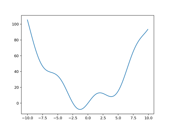
from scipy import optimize

# Function to be optimized
def f(x):
    return x**2 + 10*np.sin(x)

# Optimize w/ initial guess of 0
optimize.minimize(f, x0=0.)
  message: Optimization terminated successfully.
  success: True
   status: 0
      fun: -7.945823375615206
        x: [-1.306e+00]
      nit: 5
      jac: [-1.192e-06]
 hess_inv: [[ 8.589e-02]]
     nfev: 12
     njev: 6
Scientific Computing#
Physical phenomena can be modelled mathematically
In many cases, these mathematical models take the form of differential equations
Less commonly, they take the form of integral equations or integro-differential equations
Numerical methods convert these idealized mathematical models into a linear system of equations
The linear systems of equations are solved using linear algebra packages
Examples of commonly used numerical methods:
Finite difference method (FDM)
Finite element method (FEM)
Finite volume method (FVM)
Molecular dynamics (MD)
Density functional theory (DFT)
…
High-level programming languages like Matlab and Python (via scipy) provide an interface to the linear algebra packages written in C or Fortran
Engineering design problems require a physical quantity (e.g., weight, cost, stiffness) to be optimized given specific constraints on other physical quantities (e.g., weight, max stress)
Optimization procedures from libraries such as
scipy.optimizeor Matlab are used to solve such design problems
In some engineering scenarios, experiments are used to build a mathematical model from noisy data
Statistics and interpolation (a specific kind of optimization) are employed
scipy.interpolateandscipy.statisticsprovide interpolation algorithms and statistical functions, respectivelyR, Matlab/Octave and Julia provide alternate options
Step-by-step approach to devising a numerical model
Understand
the physics
the parameters (e.g., material properties, geometry), and
the observables (e.g., temperature, displacements, velocities)
Identify or develop the mathematical model of the physical phenomenon
E.g., Newton’s law, Schrodinger’s equation, Navier-Stokes equations, Maxwell’s equations
Create simplifying assumptions
Synthesize a computational model using various programming concepts and libraries such as numpy, scipy, as necessary
Verify the model for correctness
Correctness of a Computational Model#
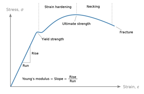
Phenomenologically correct
Example: materials are assumed to have a linear response to an applied strain – generalized Hooke’s law
This assumption holds true for small strains and breaks down at finite strains
Methodologically correct
Example: numerical approximation of the derivative of a function 𝑓(𝑥):
\(\frac{df(x)}{dx}\approx \frac{f(x+h) - f(x)}{h}\)ℎ cannot be too small or too large
𝑓 should be a well-behaved function
If neither of these conditions are met, the approximate derivative will not be correct affecting the whole computational model
Numerically correct
Example: numerical errors due to finite precision of floating-point numbers
3*0.1 == 0.3
3*0.1
A robust approach is needed to get around such issues
3*0.1 - 0.3 < 1e-8
Sympy#
Stands for symbolic Python
Allows for symbolic equation manipulation
Useful for solving symbolically:
Systems of equations
Integrals and Derivatives
Limits
Differential equations
Symbolic variables must be defined with the
symbolsfunctionEquations are defined with the
EqfunctionEquations and systems can be solved with the
solvefunction
Example: system of equations
\(x+y = 5\)
\(x = y - 3\)
import sympy as sp

x, y = sp.symbols('x y') # commas or spaces can be used
eqn1 = sp.Eq(x + y, 5)
eqn2 = sp.Eq(x, y - 3)
sol = sp.solve([eqn1, eqn2], [x, y])
print(sol)
{x: 1, y: 4}
Example: multiple solutions
\(x+y = 5\)
\(x^2 + y^2 = 17\)
eqn2 = sp.Eq(x**2 + y**2, 17)
sol = sp.solve([eqn1, eqn2],[x, y])
print(sol)
[(1, 4), (4, 1)]
Example: statics problem
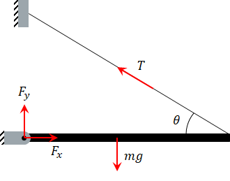
Fx, Fy, T = sp.symbols('F_x, F_y, T')
mg, th = sp.symbols('mg, theta')

# Fx - cos(th) T = 0
eq1 = sp.Eq(Fx - sp.cos(th)*T, 0)

# Fy + sin(th) T = mg
eq2 = sp.Eq(Fy + sp.sin(th)*T, mg)

# sin(th) T = mg/2
eq3 = sp.Eq(2*sp.sin(th)*T, mg)
sol = sp.solve([eq1, eq2, eq3], [Fx, Fy, T])
print(sol)
{F_x: mg*cos(theta)/(2*sin(theta)), F_y: mg/2, T: mg/(2*sin(theta))}
from IPython.display import display, Math

for item in sol.items():
    display(Math(sp.latex(item[0]) + " = " + \
            sp.latex(sp.simplify(item[1]))))        # Formats the ouput using LaTex (or its web versions KaTex in VS Code and MathJax in a browser) - a typesetting system
sp.simplify- simplifies the symbolic expression
for item in sol.items():
    num_val = item[1].subs(((mg, 1000), (th, np.pi/6))) # Input is a dictionary or a sequence
    print(f"{item[0]} = {num_val:.2f}")
F_x = 866.03
F_y = 500.00
T = 1000.00
var.subsmethod takes a dictionary or sequence of 2-tuples as input and substitutes the symbols with numeric valuesvar.evalfmethod numerically evaluates symbolic expressions
Integration and Differentiation in Sympy#
Use the
diffandintegratefunctionsdiffcan also perform partial derivatives
expr = y*x**2 + x*y**y + 1
expr
x_diff = sp.diff(expr, x)
x_diff
y_diff = sp.diff(expr, y)
y_diff
x_int = sp.integrate(expr, x)
x_int