Interpolation

Interpolation#

Assume, we have a function \(y(x)\) that is sampled at \(n\) discrete points \({x_1, x_2, \cdots, x_n}\) with high accuracy
- This data could be obtained from experiments or simulations (e.g., FDM, FEM)

How to evaluate \(y(x^*)\) where \(x_i < x^* < x_j\) (\(1\le i \lt j\le n\))?
- Use interpolation

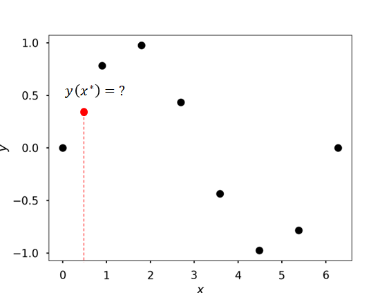
Interpolation is the process of contructing a function \(\hat{y}(x)\) that is exact at the sampled points and approximates the function elsewhere
- \(\hat{y}(x)\) is the interpolation function

Interpolation Types#

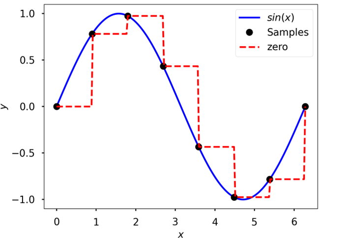
Piecewise constant
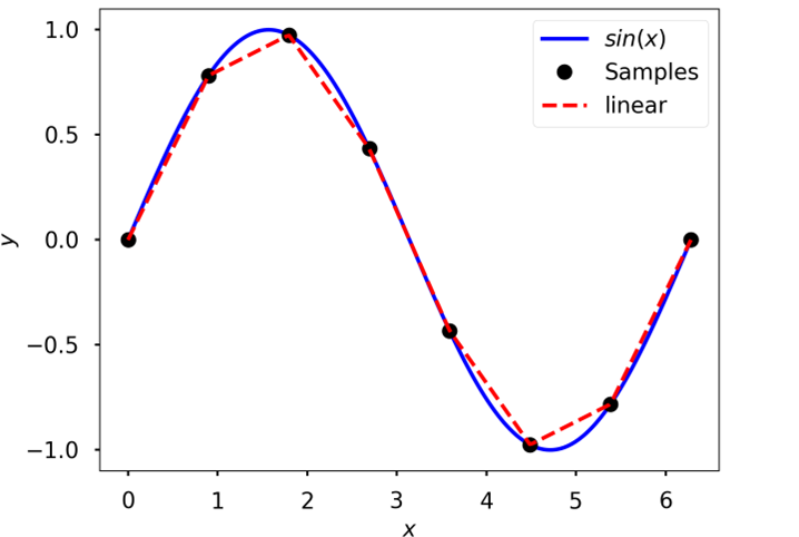
Linear
Quadratic
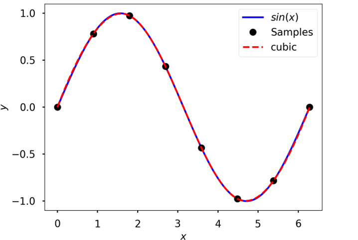
Cubic spline
Higher-order splines
…

Piecewise constant interpolation of data sampled from \(sin(x)\)

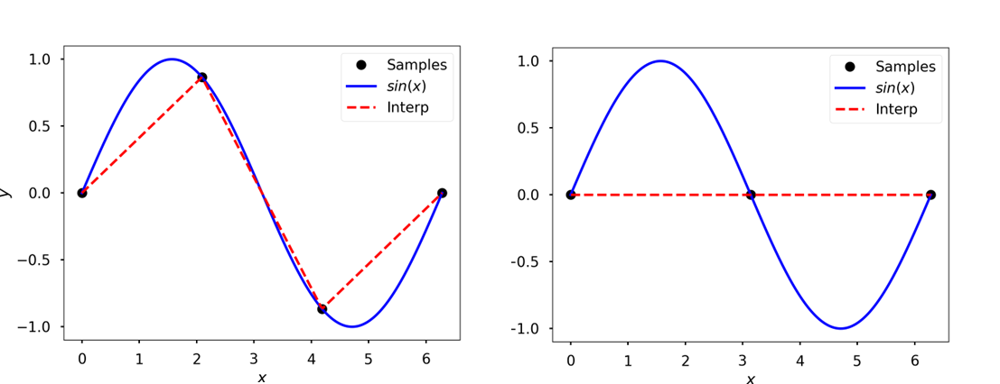
Linear interpolation of data sampled from \(sin(x)\)

Cubic interpolation of data sampled from \(sin(x)\)

Key assumption: input data has adequate information to construct an interpolation function that is sufficiently accurate
- Fewer samples \(\implies\) poor interpolation

Interpolation with four samples (left) and three samples (right)

_images/few_samples_poor_interpolation.png

The scipy sub-module interpolate provides classes for interpolation
- Univariate interpolation (1D data)
  - interp1d
  - InterpolatedUnivariateSpline
  - \(\cdots\)
- Multivariate interpolation
  - 2D data
    - interp2d
    - BivariateSpline and derived classes
    - \(\cdots\)
  - \(n\)D data
    - interpn

Refer to documentation for more details

Example#

Find an interpolation function for sampled data from \(sin(x)\)

%matplotlib widget
import numpy as np
from scipy import interpolate
import matplotlib.pyplot as plt

# Sampled data from sin
xs = np.linspace(0, 2*np.pi, 8)
ys = np.sin(xs)

---------------------------------------------------------------------------
ModuleNotFoundError                       Traceback (most recent call last)
Cell In[1], line 1
----> 1 get_ipython().run_line_magic('matplotlib', 'widget')
      2 import numpy as np
      3 from scipy import interpolate

File /opt/hostedtoolcache/Python/3.11.9/x64/lib/python3.11/site-packages/IPython/core/interactiveshell.py:2480, in InteractiveShell.run_line_magic(self, magic_name, line, _stack_depth)
   2478     kwargs['local_ns'] = self.get_local_scope(stack_depth)
   2479 with self.builtin_trap:
-> 2480     result = fn(*args, **kwargs)
   2482 # The code below prevents the output from being displayed
   2483 # when using magics with decorator @output_can_be_silenced
   2484 # when the last Python token in the expression is a ';'.
   2485 if getattr(fn, magic.MAGIC_OUTPUT_CAN_BE_SILENCED, False):

File /opt/hostedtoolcache/Python/3.11.9/x64/lib/python3.11/site-packages/IPython/core/magics/pylab.py:103, in PylabMagics.matplotlib(self, line)
     98     print(
     99         "Available matplotlib backends: %s"
    100         % _list_matplotlib_backends_and_gui_loops()
    101     )
    102 else:
--> 103     gui, backend = self.shell.enable_matplotlib(args.gui.lower() if isinstance(args.gui, str) else args.gui)
    104     self._show_matplotlib_backend(args.gui, backend)

File /opt/hostedtoolcache/Python/3.11.9/x64/lib/python3.11/site-packages/IPython/core/interactiveshell.py:3665, in InteractiveShell.enable_matplotlib(self, gui)
   3662     import matplotlib_inline.backend_inline
   3664 from IPython.core import pylabtools as pt
-> 3665 gui, backend = pt.find_gui_and_backend(gui, self.pylab_gui_select)
   3667 if gui != None:
   3668     # If we have our first gui selection, store it
   3669     if self.pylab_gui_select is None:

File /opt/hostedtoolcache/Python/3.11.9/x64/lib/python3.11/site-packages/IPython/core/pylabtools.py:338, in find_gui_and_backend(gui, gui_select)
    321 def find_gui_and_backend(gui=None, gui_select=None):
    322     """Given a gui string return the gui and mpl backend.
    323 
    324     Parameters
   (...)
    335     'WXAgg','Qt4Agg','module://matplotlib_inline.backend_inline','agg').
    336     """
--> 338     import matplotlib
    340     if _matplotlib_manages_backends():
    341         backend_registry = matplotlib.backends.registry.backend_registry

ModuleNotFoundError: No module named 'matplotlib'

# Cubic spline interpolation
f1 = interpolate.interp1d(xs, ys, kind = 'cubic')

# Alternate approach
f2 = interpolate.InterpolatedUnivariateSpline(xs, ys, k = 3)

f1 and f2 are both callable objects and can be treated as any other Python function

Using the interpolation function beyond the bounds of the sampled data will cause an error

# Interpolated data
x = np.linspace(0, 2*np.pi, 100)
y1 = f1(x)
y2 = f2(x)

# Plot
fig, axs = plt.subplots(2, 1)
axs[0].plot(x, y1, '-r', label='interp1d')
axs[1].plot(x, y2, '-r', label='UnivariateSpline')
for ax in axs:
    ax.plot(xs, ys, 'ok', markersize=6, label='Samples')
    ax.plot(x, np.sin(x), '--b', label='sin(x)')
    ax.legend();

Curve Fitting#

Given noisy data, what is the best mathematical model (i.e., function) that fits the data?

Least squares fitting, or regression, is a common approach
- Minimizes the squared error in the predicted values of the best fit \(\hat{y}\) and the actual values \(y\)

\[ E = \sum\limits_{i=0}^n \left( \hat{y}(x_i) - y(x_i) \right)^2 \]

The unknown model can be written as:

\[ \hat{y} = f(x, a_0, a_1, \cdots, a_j) \]

Here, \(f\) is a known function with \(a_0, a_1, \cdots, a_j\) being unknown coefficients to be determined by minimizing the error \(E\)

If the mathematical model \(f\) is a polynomial, it is referred to as linear regression

Curve fitting in numpy and scipy
- np.linalg.lstsq
  - Works for mathematical models of the form: \( \hat{y}(x) = \sum\limits_{i=0}^n a_i f_i(x)\)
  - Minimizing the error in this case is equivalent to solving a linear system with \(a_i\) being the unknowns

Fitting with polynomial functions
- np.polynomial subpackage provides modules for working special polynomial functions like
  - Polynomial
  - Chebyshev
  - Lagrange
  - Legendre
  - Laguerre
  - \(\cdots\)

Fitting with splines
- scipy.interpolate.UnivariateSpline class

Fitting with scipy.optimize
- optimize.curve_fit which internally uses optimize.least_squares
- Allows non-linear least squares fit

Example#

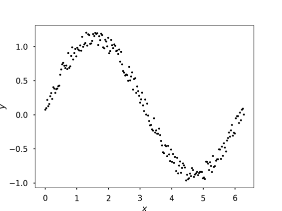
Fit data sampled from \(sin\) with added noise

# Seed for random numbers
np.random.seed(2412023)

# Data with noise - typically obtained from experiments
x = np.linspace(0, 2*np.pi, 200)
y = np.sin(x) + 0.25*np.random.rand(len(x))

Curve fitting with the model \(\hat{y}(x) = a_0 + a_1 sin(x) + a_2 cos(x)\)

For an arbitrary point \(x_i\) with a function value of \(y_i\), we have:

\[ y_i = a_0 + a_1 sin(x_i) + a_2 cos(x_i) \]

This gives us \(n\) equations in \(a_0, a_1\), and \(a_2\) (\(n\) = number of samples)

# Least squares fit
A = np.vstack([np.ones_like(x),
               np.sin(x),
               np.cos(x)]).T
fit = np.linalg.lstsq(A, y)
fit[0] # ignore the warning

# Fitted curve
y_fit = fit[0][0] + fit[0][1]*np.sin(x) + fit[0][2]*np.cos(x)

# Plot
def plot_fit(x_fit, y_fit, lbl='Fit'):
    fig, ax = plt.subplots()
    ax.plot(x, y, 'ok', markersize=2, label="Samples")
    ax.plot(x_fit, y_fit, '-r', label=lbl)
    ax.set(xlabel='x', ylabel='y')
    ax.legend();

plot_fit(x, y_fit, "Least Squares Fit")

Fit with a 6^th degree polynomial

# Least squares polynomial fit of order 6
fitPoly = np.polynomial.Polynomial.fit(x, y, 6)
print(fitPoly)

# Plot
x_fit, y_fit = fitPoly.linspace()
plot_fit(x_fit, y_fit, "Polynomial Fit")

Fit with a 6^th degree Laguerre polynomials

# Least squares Laguerre polynomial fit of order 6
fitLaguerre = np.polynomial.Laguerre.fit(x, y, 6)
print(fitLaguerre)

# Plot
x_fit, y_fit = fitLaguerre.linspace()
plot_fit(x_fit, y_fit, "Laguerre Poly Fit")

Fit with a spline function

# Spline fitting
fitSpline = interpolate.UnivariateSpline(x, y)

# Interpolation function
yHat = fitSpline(x)

# Plot
plot_fit(x, yHat, "Spline fit")

Fitting using the optimize sub-module
- Needs a prescribed mathematical model

\[ \hat{y}(x) = a_0 + a_1 sin(k_1 x) + a_2 cos(k_2 x) \]

Unlike the linalg.lstsq function, the model can be non-linear

from scipy import optimize

# Model function - can be non-linear
def model_func(x, a0, a1, k1, a2, k2):
    return a0 + a1*np.sin(k1*x) + a2*np.cos(k2*x)

# Fit
optPar, covPar = optimize.curve_fit(model_func, x, y)
optPar # Optimized parameters

# Plot
y_fit = model_func(x, optPar[0], optPar[1], optPar[2], optPar[3], optPar[4])
plot_fit(x, y_fit, "Nonlinear least squares fit")

References#

Interpolation
- https://pythonnumericalmethods.berkeley.edu/notebooks/chapter17.00-Interpolation.html
Regression/curve fitting
- https://pythonnumericalmethods.berkeley.edu/notebooks/chapter16.00-Least-Squares-Regression.html

Interpolation

Contents

Interpolation#

Interpolation Types#

Example#

Curve Fitting#

Example#

References#